LSQR-CUDA
Overview
LSQR-CUDA is written by Lawrence Ayers under the supervision of Stefan Guthe of the GRIS institute at the Technische Universität Darmstadt. It is a CUDA port of the LSQR algorithm of Chris Paige and Michael Saunders
The goal of this work was to accelerate the computation time of the well-known LSQR algorithm using a CUDA-capable GPGPU.
LSQR was first authored by Chris Paige and Michael Saunders in their publication here.
Requirements
LSQR-CUDA has the following requirements:
- *nix system or WSL for windows machines
- CUDA Capable GPGPU
- CUDA (nvcc) v11 or higher
- g++ v11 or higher
- make
Execution
To run the solver, enter the source directory and type the following command into your terminal
make run
NOTE: Before compiling, please check your GPUs compute capability. It is currently set to sm_50 in the Makefile. For best results, change this to match the capability of your GPU hardware.
Inputs
You will then be asked if you would like automatic test inputs generated for you and the desired degree sparsity of A. The range of auto-generated inputs is set in the start, end, and iteration variables of main.cu, but can be manually changed if desired. While the current setup will only build square matrices, the main.cu file can easily be modified to generate rectangular matrices.
If you have your own inputs available, you will need to save them as files with .mat (dense and sparse matrices) and .vec (vectors) extensions in the input directory. These must use a white space delimiter: “ “, and each have an appropriate number of values such that Ax=b can be satisfied.
Inputs should have the following notation:
#Arows_#Acols_A_#sparsity.mat#Arows_1_b.vec
As an example, a sparse matrix A with 1500 rows, 2000 columns, and a sparsity of 0.75% would have the following input files:
1500_2000_A_75.mat1500_1_b.vec
Outputs
The solution, x, will be written to output in a directory corresponding to the time of execution (Year-Month-DayTHourMinute) in the format:
YYYY-MM-DDTHHMM/#Acols_1_x_implementation.vec
for the above example, the x output file would look like this:
YYYY-MM-DDTHHMM/2000_1_x_CUDA-SPARSE.vec
The 5 different implementations created for this work will then run on each set of inputs located in the input directory, with the runtime of each saved to a CSV file called YYYY-MM-DDTHHMM/YYYY-MM-DDTHHMM_LSQR-CUDA.csv
___
Table of Contents
* [1. Introduction](#Introduction) * [2. Background](#Background) * [3. Methods](#Methods) * [3.1. Cpp-DENSE](#Cpp-DENSE) * [3.2. CUDA-DENSE](#CUDA-DENSE) * [3.3. CUDA-SPARSE](#CUDA-SPARSE) * [3.4. cuBLAS-DENSE](#cuBLAS-DENSE) * [3.5. cuSPARSE-SPARSE](#cuSPARSE-SPARSE) * [4. Results](#Results) * [4.1. Speedup](#Speedup) * [4.2. Accuracy](#Accuracy) * [5. Conclusion](#Conclusion)1. Introduction
The purpose of this work is to implement the LSQR algorithm on a CUDA-capable GPU to analyze any potential runtime speedups in comparison to standard, sequential CPU implementations. When run in CUDA, many matrix operations (e.g. multiplication, euclidean norm, addition, subtraction, etc.) can be run in parallel, and can, therefore, decrease computation time.
This work has both sequential and parallel implementations of LSQR that are intended for both sparse and dense inputs. The 5 implementations are, correspondingly listed as follows:
| Implementation | Matrix A | Vector b | Hardware |
|---|---|---|---|
| Cpp-DENSE | dense | dense | CPU |
| CUDA-DENSE | dense | dense | GPU |
| CUDA-SPARSE | sparse (CSR) | dense | GPU |
| cuBLAS-DENSE | dense | dense | GPU |
| cuSPARSE-SPARSE | sparse (CSR) | dense | GPU |
The implementations with DENSE in their name are those that keep A in a dense format, and, therefore, require more computation time. Those named with SPARSE first compress A into compressed sparse row (CSR) format before running. This saves execution time and memory, but requires different methods to run LSQR.
A sparse input, sequential algorithm is not explicitly created for this work, rather, the robust scipy-lsqr python solver is used instead as the baseline for verifying accuracy and comparing runtimes of the implementations made in this work.
2. Background
The LSQR algorithm is an iterative method used to find the solution x for either of the following problems:
Ax=bmin(||Ax-b||)
where A is a large, often sparse, square or rectangular matrix, and b is a vector of size A_ROWS.
LSQR was first authored by Chris Paige and Michael Saunders in their publication here, and has since been widely used for various applications.
3. Methods
The LSQR algorithm in this work is largely based off the scipy-lsqr source code as well as the C++ port provided by Luis Ibanez. In this work, the general LSQR algorithm is located in lsqr.hpp, whereby each implementation (listed above) is passed to the function as a combination of different class types (via a template).
CPU Implementations
3.1. Cpp-DENSE
The Cpp-Dense implementation is written in C++ and runs sequentially on the CPU. This implementation uses naive operations for add, subtract, multiply, Dnrm2, etc. It is the slowest of the implementations and used as a baseline to compare to dense-input GPU implementations (i.e. CUDA-DENSE and cuBLAS-DENSE). Corresponding source files are vectorCPU.cpp and vectorCPU.hpp
scipy-lsqr
Scipy’s LSQR solver is used in this work as a baseline to compare to the sparse input LSQR-CUDA implementations (i.e. CUDA-SPARSE and cuSPARSE-SPARSE). It first compresses A into CSR form before running a max of 2*A_COLUMNS iterations before returning a solution. Related information can be found on scipy’s website, and its use in this work can be found in lsqr.py
GPU Implementations
All source files pertaining to the four GPU implementations created in this work can be found in in the gpu directory.
For all CUDA kernels designed in this work, the blocksize (i.e. the number of threads in a block) is set to a constant value found in utils.cuh. This value can be changed if desired. For the GPU used in this work (NVIDIA GeForce 940M), a blocksize of 16*16 (256) threads provided best results.
The kernels used for these implementations are where most development time for LSQR-CUDA were spent.
3.2. CUDA-DENSE
The CUDA-DENSE implementation is written with the standard CUDA library, and executes many of its own kernels for various vector operations. This implementation has two dense inputs of type VectorCUDA and runs them through LSQR with accelerated multiplication, addition/subtraction, euclidean norm, and transpose operations. All operations used for this implementation are defined within the VectorCUDA class.
An output of nvprof for test-run (2500_2500_A_0.mat) of this implementation can be seen here:
nvprof output of CUDA-DENSE
``` Type Time(%) Time Calls Avg Min Max Name GPU activities: 98.00% 66.9277s 9941 6.7325ms 6.6156ms 7.4214ms multiplyTiled(double*, unsigned int*, unsigned int*, double*, unsigned int*, unsigned int*, double*) 0.51% 351.46ms 34792 10.101us 8.8320us 34.528us scale(double*, double, double*, unsigned int*, unsigned int*, bool) 0.33% 225.62ms 19880 11.349us 8.8960us 32.864us add(double*, double*, unsigned int*, unsigned int*, double*, bool) 0.33% 223.22ms 64615 3.4540us 2.7840us 3.6601ms [CUDA memset] 0.29% 197.12ms 159068 1.2390us 864ns 30.217ms [CUDA memcpy HtoD] 0.20% 137.70ms 14912 9.2340us 8.8000us 32.513us dnrm2(double*, unsigned int, unsigned int, double*, double*) 0.14% 96.548ms 34802 2.7740us 1.7600us 23.009us [CUDA memcpy DtoD] 0.13% 87.822ms 14912 5.8890us 5.0230us 26.016us maxVal(double*, unsigned int, unsigned int, double*) 0.06% 37.655ms 29827 1.2620us 1.1200us 25.344us [CUDA memcpy DtoH] 0.01% 7.9884ms 1 7.9884ms 7.9884ms 7.9884ms transposeTiled(double*, double*, unsigned int*, unsigned int*) ```Multiplication
From the nvprof output above it is clear that the most time-intensive operation of LSQR is the matrix-vector and vector-vector multiplication operations. Since CUDA-DENSE works only with dense inputs, this operation is treated the same for both matrix-vector and vector-vector multiplication.
A naive approach to parallel multiplication is to have a each thread solve for one entry in the solution matrix, i.e. a thread accesses one row of the first input and one column of the second input from global memory to perform the dot product of these two arrays in a loop. Since the latency of global memory accesses can be quite high, a cached, “tiled”, memory solution is used instead, multiplyTiled. A multiplyNaive kernel is available for reference.
In the multiplyTiled approach to parallel matrix multiplication, inputs are first loaded into GPU-cached, (“shared”) memory, or “tiles”, that iteratively “sweep” across inputs,continuously summing up the dot product result with the running total in each iteration. Each thread works in parallel towards calculating one value in the resultant matrix. An excellent visual representation of this can be found in Penny Xu’s work, Tiled Matrix Multiplication.
In multiplyTiled, the use of cache memory halves the number of global memory accesses required for each thread in comparison to the naive approach. For a dense input matrix, A, of size 2500x2500, this implementation has a speedup of about 1.5x when switching from multiplyNaive to multiplyTiled.
Scale, Addition, and Subtraction
Due to their already low computation time within the LSQR algorithm, the scale, add, and subtract operations use naive approaches. No further development for these operations was deemed necessary.
Euclidean Norm
The euclidean norm, or Dnrm2 operation, is split into two different kernels. The first, maxVal, finds the max value within the matrix or vector, and the second, dnrm2, then divides all values by this max value whilst performing the necessary multiplication and addition operations, e.g. (a[0]/maxVal) ** 2 + (a[1]/maxVal) ** 2 + .... The norm is then found by taking the square root of the dnrm2 kernel result, before multiplying it by the max-value found in the previous kernel. This is the same method used by Ibanez in LSQR-cpp and ensures numerical stability.
Standard, parallel reduction techniques are used for both of these kernels, whereby the number of working threads in a block is halved in each iteration, and memory accesses are coalesced. Much of the development here is inspired by Mark Harris’ webinar, “Optimizing Parallel Reduction in CUDA” and the topics covered in the PMPP course at TUD. Both these kernels also utilize cache memory as to decrease memory access latency.
Matrix Transpose
Like the multiplication operation, the matrix transpose operation, transposeTiled, also utilizes a “tiled” approach, where a cached “tile” is swept across the matrix iteratively transposing it section by section. While the multiplyTiled kernel requires two separate tiles (one for each input), transposeTiled requires only one that temporarily stores a section of the matrix before loading it to global memory with swapped indices, e.g. output[3][2]=input[2][3]. This method is outlined in NVIDIA’s blog post, “An Efficient Matrix Transpose in CUDA C/++”, authored by Mark Harris.
3.3. CUDA-SPARSE
The CUDA-SPARSE implementation is written with the standard CUDA library, and has inputs of type MatrixCUDA (matrix A) and VectorCUDA (vector b). When loading A into MatrixCUDA, it is converted into compressed sparse row (CSR) form, reducing its size and, depending on its sparsity, required memory and computation effort.
All operations used here are the same as the CUDA-DENSE implementation besides the matrix-vector multiplication and matrix transpose operations. These sparse matrix operations can all be found within the MatrixCUDA source code.
nvprof output of CUDA-SPARSE
``` Type Time(%) Time Calls Avg Min Max Name GPU activities: 97.49% 56.2308s 9947 5.6530ms 5.6171ms 5.6886ms spmvCSRVector(unsigned int*, int*, int*, double*, double*, double*) 0.60% 346.90ms 34813 9.9640us 8.8630us 31.328us scale(double*, double, double*, unsigned int*, unsigned int*, bool) 0.39% 225.51ms 19892 11.336us 8.8000us 34.208us add(double*, double*, unsigned int*, unsigned int*, double*, bool) 0.39% 225.08ms 64657 3.4810us 2.6880us 3.6540ms [CUDA memset] 0.37% 211.50ms 159166 1.3280us 863ns 30.498ms [CUDA memcpy HtoD] 0.24% 137.06ms 14921 9.1850us 8.7670us 30.495us dnrm2(double*, unsigned int, unsigned int, double*, double*) 0.17% 95.903ms 34823 2.7540us 2.1440us 23.008us [CUDA memcpy DtoD] 0.15% 87.760ms 14921 5.8810us 5.0230us 28.544us maxVal(double*, unsigned int, unsigned int, double*) 0.07% 37.599ms 29846 1.2590us 1.1200us 14.752us [CUDA memcpy DtoH] 0.04% 22.277ms 3 7.4258ms 7.3831ms 7.4588ms void cub::DeviceRadixSortDownsweepKernel<cub::DeviceRadixSortPolicy<int, int, int>::Policy700, bool=1, bool=0, int, int, int>(cub::DeviceRadixSortPolicy<int, int, int>::Policy700 const *, cub::DeviceRadixSortDownsweepKernel<cub::DeviceRadixSortPolicy<int, int, int>::Policy700, bool=1, bool=0, int, int, int>*, bool=1 const *, cub::DeviceRadixSortDownsweepKernel<cub::DeviceRadixSortPolicy<int, int, int>::Policy700, bool=1, bool=0, int, int, int>**, bool=0*, cub::DeviceRadixSortDownsweepKernel<cub::DeviceRadixSortPolicy<int, int, int>::Policy700, bool=1, bool=0, int, int, int>**, int, int, cub::GridEvenShare<cub::DeviceRadixSortDownsweepKernel<cub::DeviceRadixSortPolicy<int, int, int>::Policy700, bool=1, bool=0, int, int, int>**>) 0.03% 18.866ms 1 18.866ms 18.866ms 18.866ms void cusparse::gather_kernel<unsigned int=128, double, double>(double const *, int const *, int, double*) 0.03% 14.797ms 2 7.3985ms 7.3967ms 7.4004ms void cub::DeviceRadixSortDownsweepKernel<cub::DeviceRadixSortPolicy<int, int, int>::Policy700, bool=0, bool=0, int, int, int>(cub::DeviceRadixSortPolicy<int, int, int>::Policy700 const *, cub::DeviceRadixSortDownsweepKernel<cub::DeviceRadixSortPolicy<int, int, int>::Policy700, bool=0, bool=0, int, int, int>*, bool=0 const *, cub::DeviceRadixSortDownsweepKernel<cub::DeviceRadixSortPolicy<int, int, int>::Policy700, bool=0, bool=0, int, int, int>**, bool=0*, cub::DeviceRadixSortDownsweepKernel<cub::DeviceRadixSortPolicy<int, int, int>::Policy700, bool=0, bool=0, int, int, int>**, int, int, cub::GridEvenShare<cub::DeviceRadixSortDownsweepKernel<cub::DeviceRadixSortPolicy<int, int, int>::Policy700, bool=0, bool=0, int, int, int>**>) 0.02% 9.9703ms 1 9.9703ms 9.9703ms 9.9703ms void cusparse::gather_kernel<unsigned int=128, int, int>(int const *, int const *, int, int*) 0.01% 5.6034ms 3 1.8678ms 1.8501ms 1.8894ms void cub::DeviceRadixSortUpsweepKernel<cub::DeviceRadixSortPolicy<int, int, int>::Policy700, bool=1, bool=0, int, int>(cub::DeviceRadixSortPolicy<int, int, int>::Policy700 const *, bool=1*, cub::DeviceRadixSortPolicy<int, int, int>::Policy700 const *, int, int, cub::GridEvenShare<cub::DeviceRadixSortPolicy<int, int, int>::Policy700 const *>) 0.01% 3.7753ms 2 1.8876ms 1.8756ms 1.8996ms void cub::DeviceRadixSortUpsweepKernel<cub::DeviceRadixSortPolicy<int, int, int>::Policy700, bool=0, bool=0, int, int>(cub::DeviceRadixSortPolicy<int, int, int>::Policy700 const *, bool=0*, cub::DeviceRadixSortPolicy<int, int, int>::Policy700 const *, int, int, cub::GridEvenShare<cub::DeviceRadixSortPolicy<int, int, int>::Policy700 const *>) 0.00% 2.3064ms 1 2.3064ms 2.3064ms 2.3064ms void cub::DeviceReduceByKeyKernel<cub::DispatchReduceByKey<int*, int*, cub::ConstantInputIterator<int, int>, int*, int*, cub::Equality, cub::Sum, int>::PtxReduceByKeyPolicy, int*, int*, cub::ConstantInputIterator<int, int>, int*, int*, cub::ReduceByKeyScanTileState<int, int, bool=1>, cub::Equality, cub::Sum, int>(int*, int, int, cub::ConstantInputIterator<int, int>, int*, int*, int, cub::Equality, cub::Sum, int) 0.00% 2.1231ms 1 2.1231ms 2.1231ms 2.1231ms void cusparse::sequence_kernel<unsigned int=128, int>(int*, int, cusparse::sequence_kernel<unsigned int=128, int>) 0.00% 1.8211ms 1 1.8211ms 1.8211ms 1.8211ms void cusparse::csr2csr_kernel_v1<unsigned int=128, unsigned int=896, int=0, int>(int const *, int const *, int, int const **) 0.00% 54.239us 5 10.847us 10.176us 11.456us void cub::RadixSortScanBinsKernel<cub::DeviceRadixSortPolicy<int, int, int>::Policy700, int>(int*, int) 0.00% 13.664us 1 13.664us 13.664us 13.664us void cusparse::merge_path_partition_kernel<unsigned int=128, unsigned int=896, int=0, int>(int const *, int, cusparse::merge_path_partition_kernel<unsigned int=128, unsigned int=896, int=0, int>, int, int*, int) 0.00% 10.880us 1 10.880us 10.880us 10.880us void cub::DeviceScanKernel<cub::DispatchScan<int*, int*, cub::Sum, int, int>::PtxAgentScanPolicy, int*, int*, cub::ScanTileState<int, bool=1>, cub::Sum, int, int>(int*, cub::Sum, int, int, int, cub::DispatchScan<int*, int*, cub::Sum, int, int>::PtxAgentScanPolicy, int*) 0.00% 5.3120us 1 5.3120us 5.3120us 5.3120us void cusparse::scatter_kernel<unsigned int=128, int=0, int, int>(int const *, int const *, int, int*) 0.00% 4.9280us 1 4.9280us 4.9280us 4.9280us void cub::DeviceCompactInitKernel<cub::ReduceByKeyScanTileState<int, int, bool=1>, int*>(int, int, int) 0.00% 3.1360us 1 3.1360us 3.1360us 3.1360us void cub::DeviceScanInitKernel<cub::ScanTileState<int, bool=1>>(int, int) ```SpMV
As before, the nvprof output above again shows that the most expensive operation used for LSQR is multiplication. In this implementation, CUDA-SPARSE, it is the sparse matrix-vector multiplication operation, or SpMV, which solves for the product between a sparse matrix in compressed format (CSR) and a vector in dense format. The result is a vector of size #A-ROWS.
Much of the work done for the SpMV operation is based off Georgi Evushenko’s medium article, Sparse Matrix-Vector Multiplication with CUDA, and Pooja Hiranandani’s report, Sparse Matrix Vector Multiplication on GPUs: Implementation and analysis of five algorithms and corresponding github repository, spmv-cuda.
Three different SpMV kernels are available for this implementation
While the first, spmvNaive, uses one thread per row in matrix A to solve for a value in the solution vector, spmvCSRVector and spmvCSRVectorShared use, instead, one warp (i.e. 32 threads) per row in matrix A. This allows for a better utilization of resources, since the naive approach can create bottlenecks if it encounters a row that is significantly more dense than others.
The biggest difference between spmvCSRVector and spmvCSRVectorShared is their use of shared memory; spmvCSRVectorShared uses shared, cached memory, while spmvCSRVector does not. There is no real significant speedup found between these kernels when used in LSQR. spmvCSRVector is set to the default in this implementation, but it can easily be switched via the kern variable used in matrixCUDA.cu.
The run time of LSQR when using each kernel can be seen in the table below (inputs 2500_2500_A_0.mat and 2500_1_b.vec):
| kernel used | calculation time (s) |
|---|---|
| spmvNaive | 198.099 |
| spmvCSRVector | 61.102 |
| spmvCSRVectorShared | 60.198 |
cuSPARSE Transpose
The transpose of a CSR matrix is its compressed sparse column, CSC, counterpart. A kernel for this operation was not explicitly developed for this work, as it is difficult to design and/or find a good parallel implementation for it.
Also, as can be seen from the nvprof output, the transpose operation is only called once within the entire LSQR algorithm. It was, therefore, not seen as high priority seeing as it would have little impact on overall speedup.
Therefore, the existing cusparseCsr2cscEx2 function within the cuSPARSE library is used. This implementation can be found in matrixCUDA.cu More information regarding the cuSPARSE library can be found within the CUDA toolkit documentation.
3.4. cuBLAS-DENSE
The cuBLAS-DENSE implementation is written using both the CUDA and cuBLAS. cuBLAS is a library from NVIDIA that provides “basic linear algebra” operations on a GPU. For this implementation, two dense inputs of type VectorCUBLAS are used.
Information regarding cuBLAS and how to use it is documented extensively in the CUDA toolkit documentation, and will, therefore, not be further discussed here.
To see how these cuBLAS operations were used for this implementation, please refer to the VectorCUBLAS source files
3.5. cuSPARSE-SPARSE
The cuSPARSE-SPARSE implementation is written using both CUDA, cuBLAS, and cuSPARSE libraries. cuSPARSE is a library from NVIDIA that provides “a set of basic linear algebra subroutines used for handling sparse matrices”. For this implementation, one sparse input of type MatrixCUSPARSE (matrix A) and one dense input of type VectorCUBLAS (vector b) are used.
This implementation uses all the same operations as the cuBLAS-DENSE implementation, besides the SpMV and matrix transform operations, which are both executed using the cuSPARSE library. Information regarding cuBLAS and how to use it is documented extensively in the CUDA toolkit documentation, and will, therefore, not be further discussed here.
To see how these cuSPARSE operations were used for this implementation, please refer to the MatrixCUSPARSE source files
4. Results
To test LSQR-CUDA, randomly generated, square A-matrices of sparsity 0.8 are available, ranging from size 1000x1000 to 8000x8000, as well as their corresponding dense, b-vectors (sizes 1000 to 8000). These inputs can be found in the inputs.zip files in results (split into two zip files due to their size). Their corresponding x-vector solutions for each implementation can be found in outputs.zip. The runtime of each implementation of LSQR-CUDA is saved to a CSV file, RUNTIMES.csv, such that they can be compared to the runtime of the baseline, scipy-lsqr solver.
The accuracy of these implementations is also measured via root mean squared error values, which are calculated against the results of the scipy-lsqr solver. RMSE values can be found in RMSE.csv.
The organization and analysis of the test data is done via the plotting.py python script, which is provided for reference.
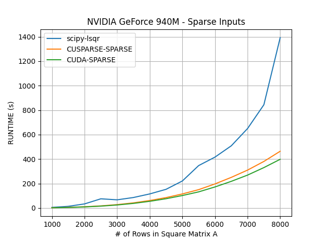
4.1. Speedup
Below, the computation time of each implementations for different sized inputs are displayed. For the following results, A_ROWS refers to the number of rows in each square A matrix, e.g. A_ROWS=1500 refers to a matrix of size A_ROWS * A_COLUMNS == 1500 * 1500 == 2150000 matrix-elements.
| A_ROWS | scipy-lsqr (SPARSE) (s) | Cpp-DENSE (s) | CUDA-DENSE (s) | CUDA-SPARSE (s) | CUBLAS-DENSE (s) | CUSPARSE-SPARSE (s) |
|---|---|---|---|---|---|---|
| 1000 | 5.36911 | 9.03528 | 6.06791 | 2.25782 | 4.23762 | 2.57307 |
| 1500 | 13.91778 | 30.57563 | 16.30271 | 4.80371 | 11.05773 | 5.59088 |
| 2000 | 33.73029 | 72.58957 | 37.55610 | 9.31562 | 22.89881 | 10.27482 |
| 2500 | 75.45058 | 342.40522 | 71.61881 | 15.67865 | 42.03487 | 17.49148 |
| 3000 | 67.19402 | 602.61113 | 115.69176 | 25.07935 | 69.78010 | 27.93229 |
| 3500 | 86.04460 | 1031.17675 | 189.35206 | 37.92124 | 108.18631 | 42.33548 |
| 4000 | 115.40540 | 1524.24163 | 281.95625 | 55.00457 | 158.94691 | 61.39182 |
| 4500 | 152.97966 | 2117.63550 | 390.68038 | 76.19237 | 224.51022 | 85.30340 |
| 5000 | 221.17113 | 2979.51575 | 548.95388 | 102.28826 | 306.09594 | 115.30341 |
| 5500 | 347.02812 | 3941.48175 | 721.66800 | 132.16242 | 400.06641 | 150.34353 |
| 6000 | 416.14977 | 5702.59200 | 928.49088 | 172.34811 | 524.00603 | 197.15688 |
| 6500 | 508.41177 | 6652.28650 | 1209.02975 | 218.11569 | 663.90925 | 250.62997 |
| 7000 | 649.83381 | 7486.82650 | 1486.45062 | 269.35181 | 824.29088 | 310.20653 |
| 7500 | 844.21635 | 9084.99600 | 1818.77300 | 330.60550 | 1011.73656 | 380.85144 |
| 8000 | 1392.32401 | 11089.35200 | 2211.38200 | 398.40791 | 1226.46113 | 464.05978 |
Sparse input implementations
The results show that the sparse input GPU implementations, CUSPARSE-SPARSE and CUDA-SPARSE, required less computation time in comparison to the scipy-lsqr solver.
Another useful metric when calculating the GPU implementations’ speeds in comparison to the scipy-lsqr solver is the “speedup” value, which is calculated by dividing CPU-runtime by GPU-runtime, i.e GPU-runtime / CPU-runtime:
| A_ROWS | CUDA-SPARSE | CUSPARSE-SPARSE |
|---|---|---|
| 1000 | 2.37800490 | 2.08665417 |
| 1500 | 2.89730134 | 2.48937383 |
| 2000 | 3.62083180 | 3.28281194 |
| 2500 | 4.81231229 | 4.31356098 |
| 3000 | 2.67925710 | 2.40560376 |
| 3500 | 2.26903461 | 2.03244638 |
| 4000 | 2.09810545 | 1.87981716 |
| 4500 | 2.00780795 | 1.79335945 |
| 5000 | 2.16223383 | 1.91816650 |
| 5500 | 2.62576999 | 2.30823447 |
| 6000 | 2.41458853 | 2.11075453 |
| 6500 | 2.33092711 | 2.02853542 |
| 7000 | 2.41258377 | 2.09484245 |
| 7500 | 2.55354598 | 2.21665527 |
| 8000 | 3.49471983 | 3.00031174 |
These values vary, but show a speedup of at least 2x for the CUDA-SPARSE implementation and 1.5x for the CUSPARSE-SPARSE implementation for all tests.
Surprisingly, the CUDA-SPARSE implementation outperformed the CUSPARSE-SPARSE implementation on all executions of LSQR. This is likely due to an error in the MatrixCUSPARSE code, as the pre-defined NVIDIA libraries often outperform CUDA kernels written from scratch. Both, however, outperformed the scipy-lsqr CPU solver and display the benefit of running LSQR on a GPU.
Dense input implementations
The dense input GPU implementations, CUDA-DENSE and CUBLAS-DENSE, were also faster than their CPU counterpart, Cpp-DENSE.
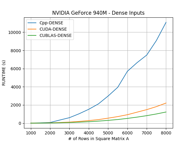
As expected, the CUBLAS-DENSE implementation outperformed the CUDA-DENSE implementation. This is likely due to the fact that CUBLAS-DENSE uses the well-optimized cuBLAS library instead of CUDA kernels written from scratch.
4.2. Accuracy
Root mean squared error (RMSE) values for both sparse and dense input GPU implementations are calculated against the results of the scipy-lsqr solver:
| A_ROWS | CUDA-DENSE | CUDA-SPARSE | CUBLAS-DENSE | CUSPARSE-SPARSE |
|---|---|---|---|---|
| 1000 | 0.00344 | 0.00024 | 0.00417 | 0.00042 |
| 1500 | 0.04059 | 0.00145 | 0.02306 | 0.00983 |
| 2000 | 0.03062 | 0.05117 | 0.06697 | 0.04953 |
| 2500 | 0.00083 | 0.00134 | 0.00060 | 0.00086 |
| 3000 | 0.00041 | 0.00012 | 0.00034 | 0.00014 |
| 3500 | 0.00015 | 0.00040 | 0.00060 | 0.00010 |
| 4000 | 0.00034 | 0.00040 | 0.00013 | 0.00119 |
| 4500 | 0.00098 | 0.00853 | 0.00739 | 0.00575 |
| 5000 | 0.00018 | 0.00058 | 0.00006 | 0.00006 |
| 5500 | 0.00042 | 0.00033 | 0.00012 | 0.00033 |
| 6000 | 0.00237 | 0.00151 | 0.00173 | 0.00230 |
| 6500 | 0.00007 | 0.00007 | 0.00004 | 0.00020 |
| 7000 | 0.01310 | 0.01141 | 0.04927 | 0.06066 |
| 7500 | 0.02260 | 0.00758 | 0.02353 | 0.01435 |
| 8000 | 0.00230 | 0.06865 | 0.04395 | 0.02216 |
All of the implementations yielded very accurate results, with none having an RMSE above 0.07.
5. Conclusion
The implementations created in this work show the benefit of running LSQR on a GPU as opposed to a CPU. For sparse input implementations, a speedup of at least 1.5x is found in comparison to that of the scipy-lsqr python solver, whilst maintaining accurate results.
This speedup, however, may not be as significant when compared to optimized LSQR-C++ solvers, like those provided by Eigen, boost, or Ibanez (as opposed to a python solver). Further research and comparison could be done here.
It should also be noted, that NVIDIA provides an LSQR solver in its cuSOLVER library, cusolverSpDcsrlsqvqr, but it currently (seemingly) only works for small datasets, and runs explicitly on the CPU. If and when NVIDIA does implement this solver for the GPU, it would be useful to compare it to the speed and accuracy of the implementations presented here.
Lastly, further measures could be taken to speedup the GPU implementations presented in this work. This could include (but is not limited to), introducing CUDA streams or using different memory allocation techniques (e.g. pinned memory) provided by CUDA. This could be potentially done in a future work.